DRL tutorial

July 17, 2023

Hey there! Welcome to this Deep Reinforcement Learning (DRL) tutorial!

During my graduate course on neural networks and deep learning at Ferdowsi University of Mashhad, under the guidance of Dr. Rouhani, I was tasked with making a presentation about deep reinforcement learning. It was a fascinating challenge to connect what we learned in class with the real-world applications of deep learning in reinforcement scenarios.

The repo containing all the files can be found here.

The slides for this tutorial can be found here!

And the gitbook is available here!

Table of contents

• 👋 Welcome to the Deep Reinforcement Learning Tutorial

The Reinforcement Learning Framework

• The Big Picture
  • RL Process
  • The reward hypothesis
• State/Observation Space
• Action Space
• Rewards and discounting
• Types of Tasks
• The Exploration/Exploitation tradeoff

Two main approaches for solving RL problems

• Policy-Based Methods
• Value-Based Methods

Value-Based Functions

• State Value Function
• Action Value Function
• The Bellman Equation

Value-Based Learning Strategies

• Monte Carlo vs Temporal Difference Learning
  • Monte Carlo: learning at the end of the episode
  • Temporal Difference Learning: learning at each step
  • Summary
• Off-policy vs On-policy
• Q-Learning
  • Introducing Q-Learning
  • The Q-Learning Algorithm

Deep Q-Learning

• From Q-Learning to Deep Q-Learning
• The Deep Q-Network (DQN)
• The Deep Q-Learning Algorithm
  • Experience Replay
  • Fixed Q-Target
  • Double DQN

Policy-Based Learning Strategies

• Introducing Policy-Gradient Methods
• The Advantages and Disadvantages of Policy-Gradient Methods
• Policy-Gradient Methods
  • The Policy-Gradient Theorem
• The Reinforce Algorithm
  • The Problem of Variance in Reinforce

Actor-Critic Methods

• Introducing Actor-Critic Methods
• The Actor-Critic Process
• Adding Advantage in Actor-Critic (A2C)

Offline Reinforcement Learning

• Offline vs. Online Reinforcement Learning
• What makes Offline Reinforcement Learning Difficult?

The Big Picture

The idea behind Reinforcement Learning is that an agent (an AI) will learn from the environment by interacting with it (through trial and error) and receiving rewards (negative or positive) as feedback for performing actions.

Formal definitions

“Reinforcement learning provides a mathematical formalism for learning-based decision making”

Reinforcement learning is an approach for learning decision making and control from experience

Reinforcement learning is a framework for solving control tasks (also called decision problems) by building agents that learn from the environment by interacting with it through trial and error and receiving rewards (positive or negative) as unique feedback.

RL Process

---

The RL Process: a loop of state, action, reward and next state

• Our Agent receives state 𝑆₀ from the Environment
• Based on that state 𝑆₀, the Agent takes action 𝐴₀
• The environment goes to a new state 𝑆₁
• The environment gives some reward 𝑅₁​ to the Agent

The agent’s goal is to maximize its cumulative reward, called the expected return.

The reward hypothesis

---

The reward hypothesis: the central idea of Reinforcement Learning

Why is the goal of the agent to maximize the expected return?

Because RL is based on the reward hypothesis, which is that all goals can be described as the maximization of the expected return (expected cumulative reward).

That’s why in Reinforcement Learning, to have the best behavior, we aim to learn to take actions that maximize the expected cumulative reward.

Markov Property

The Markov Property implies that our agent needs only the current state to decide what action to take and not the history of all the states and actions they took before.

State-Observation Space

Observations/States are the information our agent gets from the environment. In the case of a video game, it can be a frame (a screenshot). In the case of the trading agent, it can be the value of a certain stock, etc.

There is a differentiation to make between observation and state, however:

State s:

is a complete description of the state of the world (there is no hidden information). In a fully observed environment.

In a chess game, we have access to the whole board information, so we receive a state from the environment. In other words, the environment is fully observed.

Observation o:

is a partial description of the state. In a partially observed environment

In Super Mario Bros, we only see the part of the level close to the player, so we receive an observation. In Super Mario Bros, we are in a partially observed environment. We receive an observation since we only see a part of the level.

Action Space

The Action space is the set of all possible actions in an environment.

The actions can come from a discrete or continuous space:

Discrete space

The number of possible actions is finite.

Again, in Super Mario Bros, we have only 5 possible actions: 4 directions and jumping

In Super Mario Bros, we have a finite set of actions since we have only 5 possible actions: 4 directions and jump.

Continuous space

The number of possible actions is infinite.

A Self Driving Car agent has an infinite number of possible actions since it can turn left 20°, 21,1°, 21,2°, honk, turn right 20°…

Rewards and discounting

The reward is fundamental in RL because it’s the only feedback for the agent. Thanks to it, our agent knows if the action taken was good or not.

The cumulative reward at each time step t can be written as:

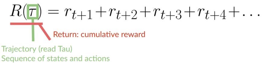
The cumulative reward equals the sum of all rewards in the sequence.

which is equivalent to:

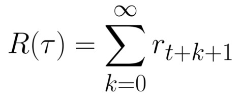
The cumulative reward = rt+1 (rt+k+1 = rt+0+1 = rt+1)+ rt+2 (rt+k+1 = rt+1+1 = rt+2) + ...

However, in reality, we can’t just add them like that. The rewards that come sooner (at the beginning of the game) are more likely to happen since they are more predictable than the long-term future reward.

---

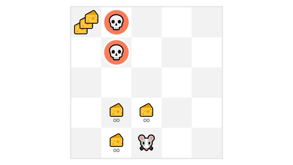
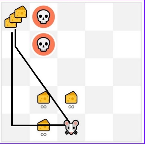
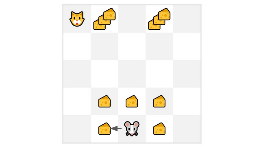
Let’s say your agent is this tiny mouse that can move one tile each time step, and your opponent is the cat (that can move too). The mouse’s goal is to eat the maximum amount of cheese before being eaten by the cat.

• As we can see in the diagram, it’s more probable to eat the cheese near us than the cheese close to the cat (the closer we are to the cat, the more dangerous it is).
• Consequently, the reward near the cat, even if it is bigger (more cheese), will be more discounted since we’re not really sure we’ll be able to eat it.

To discount the rewards, we proceed like this:

1. We define a discount rate called gamma. It must be between 0 and 1. Most of the time between 0.95 and 0.99.
   1. The larger the gamma, the smaller the discount. This means our agent cares more about the long-term reward.
   2. On the other hand, the smaller the gamma, the bigger the discount. This means our agent cares more about the short term reward (the nearest cheese).
2. Then, each reward will be discounted by gamma to the exponent of the time step. As the time step increases, the cat gets closer to us, so the future reward is less and less likely to happen.

Our discounted expected cumulative reward is:

Types of Tasks

A task is an instance of a Reinforcement Learning problem. We can have two types of tasks: episodic and continuing

Episodic task

In this case, we have a starting point and an ending point (a terminal state). This creates an episode: a list of States, Actions, Rewards, and new States.

For instance, think about Super Mario Bros: an episode begin at the launch of a new Mario Level and ends when you’re killed or you reached the end of the level.

Continuous task

These are tasks that continue forever (no terminal state). In this case, the agent must learn how to choose the best actions and simultaneously interact with the environment.

For instance, an agent that does automated stock trading. For this task, there is no starting point and terminal state. The agent keeps running until we decide to stop it.

The Exploration-Exploitation tradeoff

Remember, the goal of our RL agent is to maximize the expected cumulative reward. However, we can fall into a common trap.

• Exploration is exploring the environment by trying random actions in order to find more information about the environment.
• Exploitation is exploiting known information to maximize the reward.

Let’s take an example:

In this game, our mouse can have an infinite amount of small cheese (+1 each). But at the top of the maze, there is a gigantic sum of cheese (+1000).

If we only focus on exploitation, our agent will never reach the gigantic sum of cheese. Instead, it will only exploit the nearest source of rewards, even if this source is small (exploitation).

But if our agent does a little bit of exploration, it can discover the big reward (the pile of big cheese).

This is what we call the exploration/exploitation trade-off. We need to balance how much we explore the environment and how much we exploit what we know about the environment.

Therefore, we must define a rule that helps to handle this trade-off.

Policy-Based Methods

Now that we learned the RL framework, how do we solve the RL problem? In other words, how do we build an RL agent that can select the actions that maximize its expected cumulative reward?

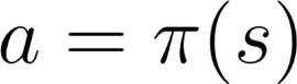
The policy π: the agent’s brain

The Policy π is the brain of our Agent, it’s the function that tells us what action to take given the state we are in. So it defines the agent’s behavior at a given time.

Think of policy as the brain of our agent, the function that will tell us the action to take given a state

This Policy is the function we want to learn, our goal is to find the optimal policy π*, the policy that maximizes expected return when the agent acts according to it. We find this π* through training.

There are two approaches to train our agent to find this optimal policy π*:

• Directly, by teaching the agent to learn which action to take, given the current state: Policy-Based Methods.
• Indirectly, teach the agent to learn which state is more valuable and then take the action that leads to the more valuable states: Value-Based Methods.

---

In Policy Based methods, we learn a policy function directly.

As we can see here, the policy (deterministic) directly indicates the action to take for each step

This function will define a mapping from each state to the best corresponding action. Alternatively, it could define a probability distribution over the set of possible actions at that state . We have two types of policies:

Deterministic:

a policy at a given state will always return the same action

action = policy(state)

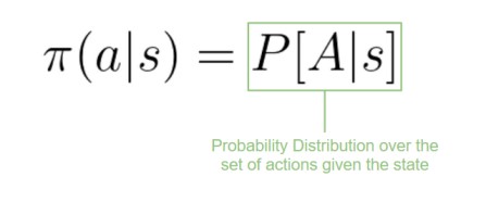
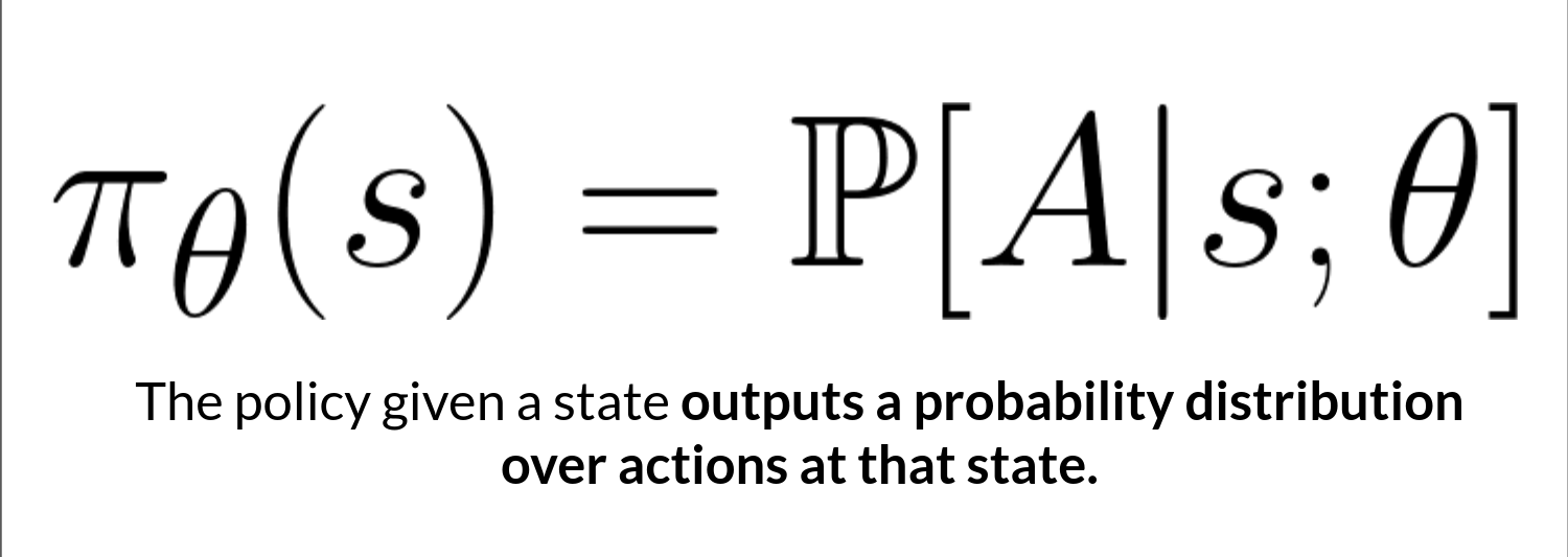
Stochastic:

outputs a probability distribution over actions.

{:style=”display:block; margin-left:auto; margin-right:auto”}
<p style="text-align: center;">policy(actions	state) = probability distribution over the set of actions given the current state</p>

Given an initial state, our stochastic policy will output probability distributions over the possible actions at that state.

Value-Based Methods

In value-based methods, instead of learning a policy function, we learn a value function that maps a state to the expected value of being at that state.

The value of a state is the expected discounted return the agent can get if it starts in that state, and then acts according to our policy.

---

But what does it mean to act according to our policy? After all, we don’t have a policy in value-based methods since we train a value function and not a policy.

Here we see that our value function defined values for each possible state.

Thanks to our value function, at each step our policy will select the state with the biggest value defined by the value function: -7, then -6, then -5 (and so on) to attain the goal.

Since the policy is not trained/learned, we need to specify its behavior. For instance, if we want a policy that, given the value function, will take actions that always lead to the biggest reward, we’ll create a Greedy Policy.

In this case, you don’t train the policy: your policy is just a simple pre-specified function (for instance, the Greedy Policy) that uses the values given by the value-function to select its actions.

In value-based training, finding an optimal value function (denoted Q* or V*) leads to having an optimal policy.

Finding an optimal value function leads to having an optimal policy.

In fact, most of the time, in value-based methods, you’ll use an Epsilon-Greedy Policy that handles the exploration/exploitation trade-off.

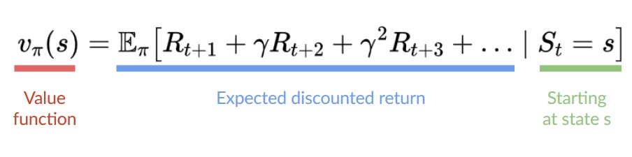
State Value Function

---

We write the state value function under a policy π like this:

For each state, the state-value function outputs the expected return if the agent starts at that state and then follows the policy forever afterward (for all future timesteps, if you prefer).

If we take the state with value -7: it's the expected return starting at that state and taking actions according to our policy (greedy policy), so right, right, right, down, down, right, right.

Action Value Function

---

The value of taking action a in state s under a policy π is:

In the action-value function, for each state and action pair, the action-value function outputs the expected return if the agent starts in that state, takes that action, and then follows the policy forever after.

We see that the difference is:

• For the state-value function, we calculate the value of a state 𝑆𝑡.
• For the action-value function, we calculate the value of the state-action pair ( 𝑆𝑡, 𝐴𝑡 ) hence the value of taking that action at that state.
• In either case, whichever value function we choose (state-value or action-value function), the returned value is the expected return.
• However, the problem is that to calculate EACH value of a state or a state-action pair, we need to sum all the rewards an agent can get if it starts at that state.
• This can be a computationally expensive process, and that’s where the Bellman equation comes in to help us.

The Bellman Equation

Instead of calculating the expected return for each state or each state-action pair, we can use the Bellman equation.

The Bellman equation is a recursive equation that works like this:

Instead of starting for each state from the beginning and calculating the return, we can consider the value of any state as:

The immediate reward 𝑅𝑡_+1** + the discounted value of the state that follows (** 𝑔𝑎𝑚𝑚𝑎∗𝑉(𝑆𝑡+1_) ) .

To recap, the idea of the Bellman equation is that instead of calculating each value as the sum of the expected return, which is a long process, we calculate the value as the sum of immediate reward + the discounted value of the state that follows.

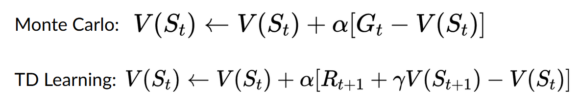
Monte Carlo vs Temporal Difference Learning

The idea behind Reinforcement Learning is that given the experience and the received reward, the agent will update its value function or policy.

Monte Carlo and Temporal Difference Learning are two different strategies on how to train our value function or our policy function. Both of them use experience to solve the RL problem.

• On one hand, Monte Carlo uses an entire episode of experience before learning.
• On the other hand, Temporal Difference uses only a step ⟮𝑆𝑡，𝐴𝑡，𝑅𝑡+1，𝑆𝑡+1⟯ to learn.

Monte Carlo: learning at the end of the episode

Monte Carlo approach:

Monte Carlo waits until the end of the episode, calculates 𝐺𝑡 (return) and uses it as a target for updating 𝑉⟮𝑆𝑡⟯.

So it requires a complete episode of interaction before updating our value function.

If we take an example:

• We always start the episode at the same starting point.
• The agent takes actions using the policy. For instance, using an Epsilon Greedy Strategy, a policy that alternates between exploration (random actions) and exploitation.
• We get the reward and the next state.
• We terminate the episode if the cat eats the mouse or if the mouse moves > 10 steps.

At the end of the episode:

• We have a list of State, Actions, Rewards, and Next States tuples.
• The agent will sum the total rewards 𝐺𝑡 (to see how well it did).
• It will then update 𝑉⟮𝑆𝑡⟯ based on the formula.
• Then start a new game with this new knowledge better.

By running more and more episodes, the agent will learn to play better and better.

---

For instance, if we train a state-value function using Monte Carlo:

• We initialize our value function so that it returns 0 value for each state.
• Our learning rate (lr) is 0.1 and our discount rate is 1 (= no discount).
• Our mouse explores the environment and takes random actions.

• The mouse made more than 10 steps, so the episode ends.
• We have a list of state, action, rewards, next_state, we need to calculate the return 𝐺𝑡.
  • 𝐺𝑡=𝑅𝑡+1+𝑅𝑡+2+𝑅𝑡+3…(for simplicity we don’t discount the rewards).
  • 𝐺𝑡=1+0+0+0+0+0+1+1+0+0Gt​=1+0+0+0+0+0+1+1+0+0
  • 𝐺𝑡=3
• We can now update 𝑉⟮𝑆0⟯:
  • New 𝑉⟮𝑆0⟯=𝑉⟮𝑆0⟯+lr∗[𝐺𝑡—𝑉⟮𝑆0⟯)]
  • New 𝑉⟮𝑆0⟯=0+0.1∗[3–0]𝑉⟮𝑆0⟯
  • New 𝑉⟮𝑆0⟯=0.3V

Temporal Difference Learning: learning at each step

Temporal Difference, on the other hand, waits for only one interaction (one step) 𝑆𝑡+1 to form a TD target and update 𝑉⟮𝑆𝑡⟯ using 𝑅𝑡+1​ and 𝛾∗𝑉⟮𝑆𝑡+1⟯.

The idea with TD is to update the 𝑉⟮𝑆𝑡⟯at each step.

But because we didn’t experience an entire episode, we don’t have 𝐺𝑡 (expected return). Instead, we estimate 𝐺𝑡 by adding 𝑅𝑡+1 and the discounted value of the next state.

This is called bootstrapping. It’s called this because TD bases its update in part on an existing estimate 𝑉⟮𝑆𝑡+1⟯ and not a complete sample 𝐺𝑡​.

TD approach:

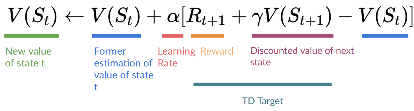
This method is called TD(0) or one-step TD (update the value function after any individual step).

TD Approach:

At the end of one step (State, Actions, Rewards, and Next States):

• We have 𝑅𝑡+1​ and 𝑆𝑡+1
• We update 𝑉⟮𝑆𝑡⟯:
  • we estimate 𝐺𝑡 by adding 𝑅𝑡+1and the discounted value of the next state.
  • TD Target: 𝑅𝑡+1​ + 𝛾∗𝑉⟮𝑆𝑡+1⟯

Now we continue to interact with this environment with our updated value function. By running more and more steps, the agent will learn to play better and better.

---

If we take an example:

• We initialize our value function so that it returns 0 value for each state.
• Our learning rate (lr) is 0.1 and our discount rate is 1 (= no discount).
• Our mouse begins to explore the environment and takes a random action: going to the left
• It gets a reward 𝑅𝑡+1​ = 1 since it eats a piece of cheese

We can now update 𝑉⟮𝑆0⟯:

• New 𝑉⟮𝑆0⟯=𝑉⟮𝑆0⟯+lr∗[𝑅1​+𝛾∗𝑉⟮𝑆0⟯−𝑉⟮𝑆0⟯]
• New𝑉⟮𝑆0⟯=0+0.1∗[1+1∗0–0]
• New𝑉⟮𝑆0⟯=0.1

So we just updated our value function for State 0.

Now we continue to interact with this environment with our updated value function.

Summary

• With Monte Carlo, we update the value function from a complete episode, and so we use the actual accurate discounted return of this episode.
• With TD Learning, we update the value function from a step, and we replace 𝐺𝑡, which we don’t know, with an estimated return called the TD target.

Off-policy vs On-policy

---

On-Policy Reinforcement Learning:

In on-policy RL, the agent learns from the experiences it gathers while following its current policy. This means that the data used for training the agent comes from the same policy it is trying to improve. It updates its policy based on its current actions and their consequences.

Key characteristics of on-policy RL:

• Data collection and policy improvement are interleaved: The agent collects data by interacting with the environment according to the current policy, and then it uses this data to update its policy.
• Can be more sample-efficient: Since it learns from its own experiences, on-policy methods can sometimes converge faster with fewer samples compared to off-policy methods.
• Tends to be more stable: As the agent is learning from its current policy, it is less likely to face issues related to distributional shift or divergence.
• However, it might be less explorative: Since it follows its current policy closely, it may not explore new actions and paths effectively.

Off-Policy Reinforcement Learning:

In off-policy RL, the agent learns from experiences generated by a different (usually older) policy, often referred to as the “behavior policy.” It uses these experiences to learn and improve a different policy called the “target policy.” This decoupling of data collection and policy improvement allows for greater flexibility.

Key characteristics of off-policy RL:

• Data collection and policy improvement are decoupled: The agent collects data by exploring the environment using a behavior policy, but it uses this data to improve a different target policy.
• Can be more explorative: Since the behavior policy can be explorative, off-policy algorithms have the potential to discover new and better actions.
• Higher potential for reusability: Once data is collected, it can be reused to train multiple target policies, making it more sample-efficient for later improvements.
• May suffer from issues with distributional shift: As the data comes from a different policy, off-policy methods need to handle potential distributional differences between the behavior policy and the target policy.

Q-Learning

---

What is Q-Learning?

Q-Learning is an off-policy value-based method that uses a TD approach to train its action-value function:

Introducing Q-Learning

• Off-policy: the epsilon-greedy policy (acting policy), is different from the greedy policy that is used to select the best next-state action value to update our Q-value (updating policy).
• Value-based method: finds the optimal policy indirectly by training a value or action-value function that will tell us the value of each state or each state-action pair.
• TD approach: updates its action-value function at each step instead of at the end of the episode.

Q-Learning is the algorithm we use to train our Q-function, an action-value function that determines the value of being at a particular state and taking a specific action at that state.

The Q comes from “the Quality” (the value) of that action at that state.

---

Let’s recap the difference between value and reward:

Value

The value of a state, or a state-action pair is the expected cumulative reward our agent gets if it starts at this state (or state-action pair) and then acts accordingly to its policy.

Reward

The reward is the feedback I get from the environment after performing an action at a state.

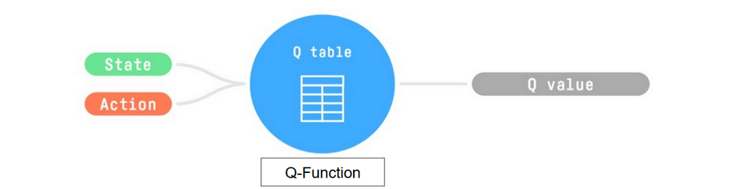
Internally, our Q-function is encoded by a Q-table, a table where each cell corresponds to a state-action pair value. Think of this Q-table as the memory or cheat sheet of our Q-function.

---

Let’s go through an example of a maze.

The Q-table is initialized. That’s why all values are = 0. This table contains, for each state and action, the corresponding state-action values.

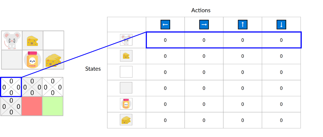
Here we see that the state-action value of the initial state and going up is 0:

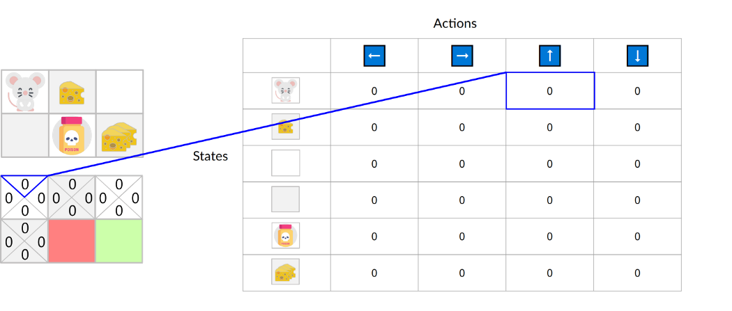
So: the Q-function uses a Q-table that has the value of each state-action pair. Given a state and action, our Q-function will search inside its Q-table to output the value.

---

If we recap, Q-Learning is the RL algorithm that:

• Trains a Q-function(an action-value function), which internally is a Q-table that contains all the state-action pair values.
• Given a state and action, our Q-function will search its Q-table for the corresponding value.
• When the training is done, we have an optimal Q-function, which means we have optimal Q-table.
• And if we have an optimal Q-function, we have an optimal policy since we know the best action to take at each state.

In the beginning, our Q-table is useless since it gives arbitrary values for each state-action pair (most of the time, we initialize the Q-table to 0).

As the agent explores the environment and we update the Q-table, it will give us a better and better approximation to the optimal policy.

The Q-Learning Algorithm

---

Step 01: We initialize the Q-table

We need to initialize the Q-table for each state-action pair. Most of the time, we initialize with values of 0.

---

Step 02: Choose an action using the epsilon-greedy strategy

The epsilon-greedy strategy is a policy that handles the exploration/exploitation trade-off.

The idea is that, with an initial value of ɛ = 1.0:

• With probability 1 —ɛ : we do exploitation (aka our agent selects the action with the highest state-action pair value).
• With probability ɛ: we do exploration (trying random action).

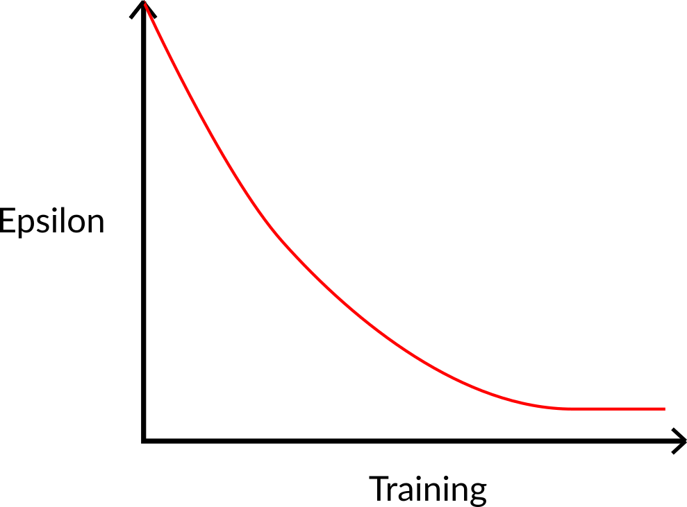
At the beginning of the training, the probability of doing exploration will be huge since ɛ is very high, so most of the time, we’ll explore. But as the training goes on, and consequently our Q-table gets better and better in its estimations, we progressively reduce the epsilon value since we will need less and less exploration and more exploitation.

---

Step 03: Perform action 𝐴𝑡, get reward 𝑅𝑡+1 and next state 𝑆𝑡+1

---

Step 4: Update 𝑄⟮𝑆𝑡, 𝐴𝑡⟯

Remember that in TD Learning, we update our policy or value function (depending on the RL method we choose) after one step of the interaction.

To produce our TD target, we used the immediate reward 𝑅𝑡+1​ plus the discounted value of the next state, computed by finding the action that maximizes the current Q-function at the next state. (We call that bootstrap).

Therefore, our 𝑄⟮𝑆𝑡, 𝐴𝑡⟯ update formula goes like this:

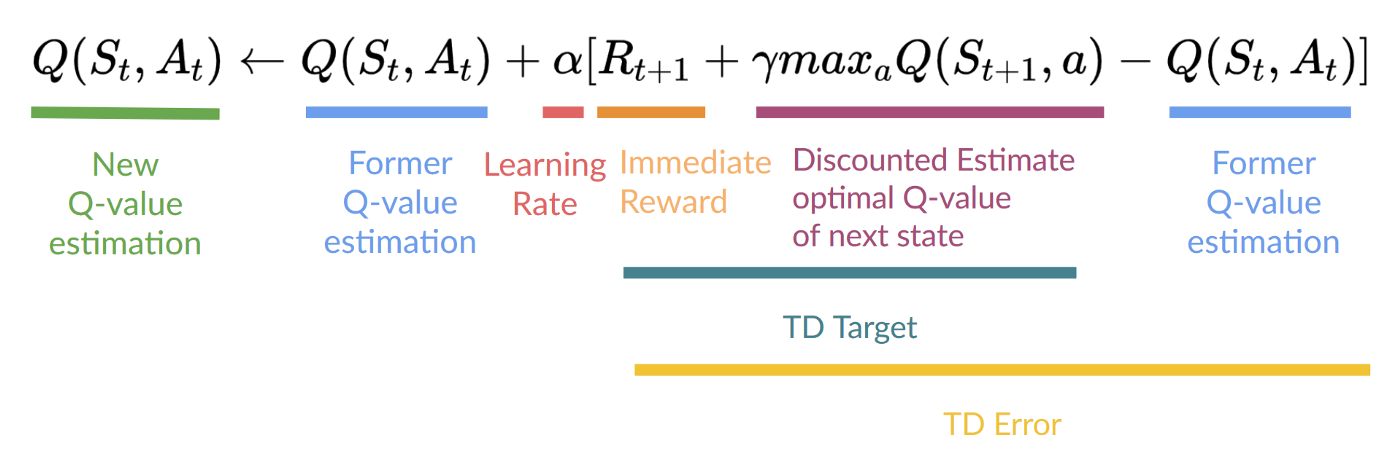
This means that to update our 𝑄⟮𝑆𝑡, 𝐴𝑡⟯:

• We need 𝑆𝑡, 𝐴𝑡, 𝑅𝑡+1, 𝑆𝑡+1
• To update our Q-value at a given state-action pair, we use the TD target.

How do we form the TD target?

1. We obtain the reward after taking the action 𝑅𝑡+1
2. To get the best state-action pair value for the next state, we use a greedy policy to select the next best action. Note that this is not an epsilon-greedy policy, this will always take the action with the highest state-action value.

Then when the update of this Q-value is done, we start in a new state and select our action using a epsilon-greedy policy again.

This is why we say that Q Learning is an off-policy algorithm.

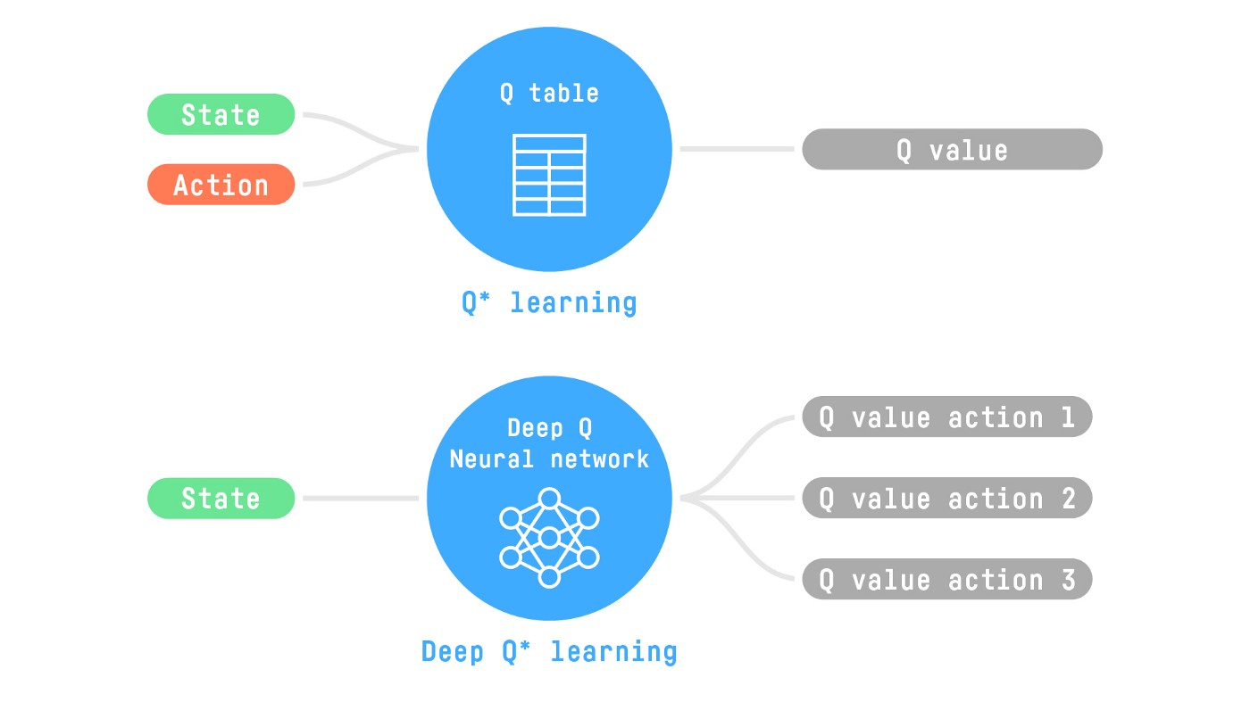
From Q-Learning to Deep Q-Learning

We learned that Q-Learning is an algorithm we use to train our Q-Function, an action-value function that determines the value of being at a particular state and taking a specific action at that state.

Internally, our Q-function is encoded by a Q-table, a table where each cell corresponds to a state-action pair value. Think of this Q-table as the memory or cheat sheet of our Q-function.

The problem is that Q-Learning is a tabular method. This becomes a problem if the states and actions spaces are not small enough to be represented efficiently by arrays and tables. In other words: it is not scalable.

• Atari environments have an observation space with a shape of (210, 160, 3)*, containing values ranging from 0 to 255 so that gives us 256^(210×160×3)=256^(100800) (for comparison, we have approximately 10801080 atoms in the observable universe).

Therefore, the state space is gigantic; due to this, creating and updating a Q-table for that environment would not be efficient. In this case, the best idea is to approximate the Q-values using a parametrized Q-function 𝑄𝜃⟮𝑠,𝑎⟯.

possible observations (for comparison, we have approximately

This neural network will approximate, given a state, the different Q-values for each possible action at that state. And that’s exactly what Deep Q-Learning does.

The Deep Q-Network (DQN)

This is the architecture of our Deep Q-Learning network:

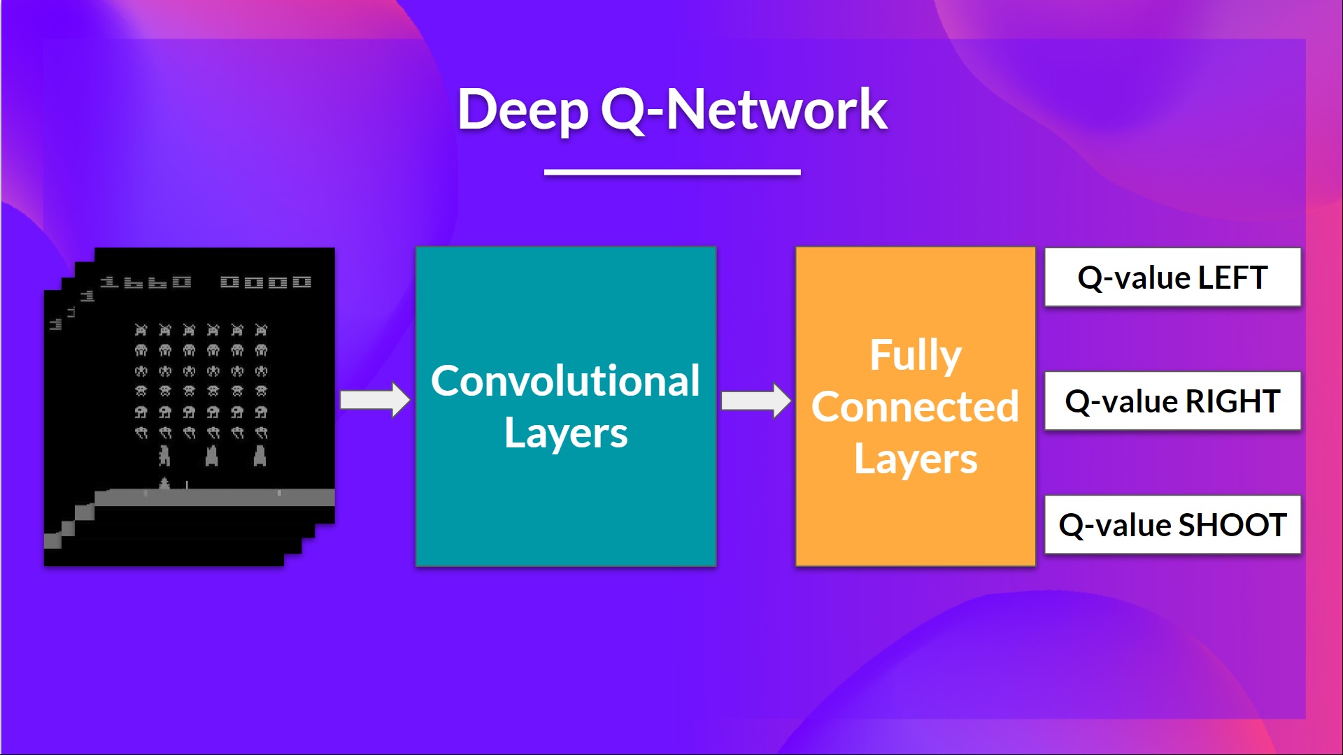
As input, we take a stack of 4 frames passed through the network as a state and output a vector of Q-values for each possible action at that state. Then, like with Q-Learning, we just need to use our epsilon-greedy policy to select which action to take.

When the Neural Network is initialized, the Q-value estimation is terrible. But during training, our Deep QNetwork agent will associate a situation with the appropriate action and learn to play the game well.

Then the stacked frames are processed by three convolutional layers. These layers allow us to capture and exploit spatial relationships in images.

Finally, we have a couple of fully connected layers that output a Q-value for each possible action at that state.

So, the Deep Q-Learning uses a neural network to approximate, given a state, the different Q-values for each possible action at that state.

---

Preprocessing the input and temporal limitation:

We need to preprocess the input. It’s an essential step since we want to reduce the complexity of our state to reduce the computation time needed for training.

1. To achieve this, we reduce the state space to 84x84 and grayscale it. This is a big improvement since we reduce our three color channels (RGB) to 1.
2. We can also crop a part of the screen in some games if it does not contain important information. Then we stack four frames together.

Why do we stack four frames together? We stack frames together because it helps us handle the problem of temporal limitation.

Let’s take an example with the game of Pong. When you see this frame:

Can you tell me where the ball is going?

No, because one frame is not enough to have a sense of motion!

But what if I add three more frames? Here you can see ball is going? Here, you can see that the ball is going to the right.

The Deep Q-Learning Algorithm

We learned that Deep Q-Learning uses a deep neural network to approximate the different Q-values for each possible action at a state (value-function estimation).

The difference is that, during the training phase, instead of updating the Q-value of a state-action pair directly as we have done with Q-Learning:

In Deep Q-Learning, we create a loss function that compares our prediction and the gradient descent to update the weights of our Deep Q-Network to approximate our Q-values better.

The Deep Q-Learning training algorithm has two phases:

1. Sampling: we perform actions and store the observed experience tuples in a replay memory.
2. Training: Select a small batch of tuples randomly and learn from this batch using a gradient descent update step.

This is not the only difference compared with Q-Learning.

Deep Q-Learning training might suffer from instability, mainly because of combining a non-linear Q-value function (Neural Network) and bootstrapping (when we update targets with existing estimates and not an actual complete return).

To help us stabilize the training, we implement three different solutions:

1.	Experience Replay to make more efficient use of experiences.
2.	Fixed Q-Target to stabilize the training.
2.	Double Deep Q-Learning, to handle the problem of the overestimation of Q-values.

Experience Replay

Why do we create a replay memory? Experience Replay in Deep Q-Learning has two functions:

Make more efficient use of the experiences during the training.

Usually, in online reinforcement learning, the agent interacts with the environment, gets experiences (state, action, reward, and next state), learns from them (updates the neural network), and discards them. This is not efficient.

Experience replay helps by using the experiences of the training more efficiently. We use a replay buffer that saves experience samples that we can reuse during the training.

This allows the agent to learn from the same experiences multiple times.

Avoid forgetting previous experiences and reduce the correlation between experiences.

The problem we get if we give sequential samples of experiences to our neural network is that it tends to forget the previous experiences as it gets new experiences. For instance, if the agent is in the first level and then in the second, which is different, it can forget how to behave and play in the first level.

The solution is to create a Replay Buffer that stores experience tuples while interacting with the environment and then sample a small batch of tuples. This prevents the network from only learning about what it has done immediately before.

Experience replay also has other benefits. By randomly sampling the experiences, we remove correlation in the observation sequences and avoid action values from oscillating or diverging catastrophically.

In the Deep Q-Learning pseudocode, we initialize a replay memory buffer D with capacity N (N is a hyperparameter that you can define). We then store experiences in the memory and sample a batch of experiences to feed the Deep Q-Network during the training phase.

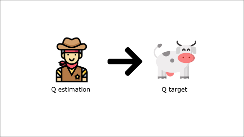
Fixed Q-Target

When we want to calculate the TD error (aka the loss), we calculate the difference between the TD target (Q-Target) and the current Q-value (estimation of Q).

But we don’t have any idea of the real TD target. We need to estimate it. Using the Bellman equation, we saw that the TD target is just the reward of taking that action at that state plus the discounted highest Q value for the next state.

Q-Target

Q-Loss

However, the problem is that we are using the same parameters (weights) for estimating the TD target and the Q-value. Consequently, there is a significant correlation between the TD target and the parameters we are changing.

Therefore, at every step of training, both our Q-values and the target values shift. We’re getting closer to our target, but the target is also moving. It’s like chasing a moving target!

This can lead to significant oscillation in training.

---

It’s like if you were a cowboy (the Q estimation) and you wanted to catch a cow (the Q-target). Your goal is to get closer (reduce the error).

At each time step, you’re trying to approach the cow, which also moves at each time step (because you use the same parameters).

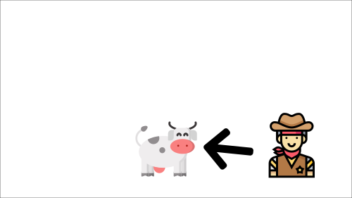
This leads to a bizarre path of chasing (a significant oscillation in training).

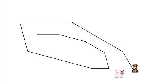
Instead, what we see in the pseudo-code is that we:

• Use a separate network with fixed parameters for estimating the TD Target
• Copy the parameters from our Deep Q-Network every C steps to update the target network.

Double DQN

Double DQNs, or Double Deep Q-Learning neural networks, were introduced by Hado van Hasselt. This method handles the problem of the overestimation of Q-values.

When calculating the TD Target, we face a simple problem: how are we sure that the best action for the next state is the action with the highest Q-value?

We know that the accuracy of Q-values depends on what action we tried and what neighboring states we explored.

Consequently, we don’t have enough information about the best action to take at the beginning of the training. Therefore, taking the maximum Q-value (which is noisy) as the best action to take can lead to false positives. If non-optimal actions are regularly given a higher Q value than the optimal best action, the learning will be complicated.

The solution is: when we compute the Q target, we use two networks to decouple the action selection from the target Q-value generation. We:

• Use our DQN network to select the best action to take for the next state (the action with the highest Q-value).
• Use our Target network to calculate the target Q-value of taking that action at the next state.

Therefore, Double DQN helps us reduce the overestimation of Q-values and, as a consequence, helps us train faster and with more stable learning.

Introducing Policy-Gradient Methods

---

Recap of Policy-Based Methods

In policy-based methods, we directly learn to approximate π∗ without having to learn a value function.

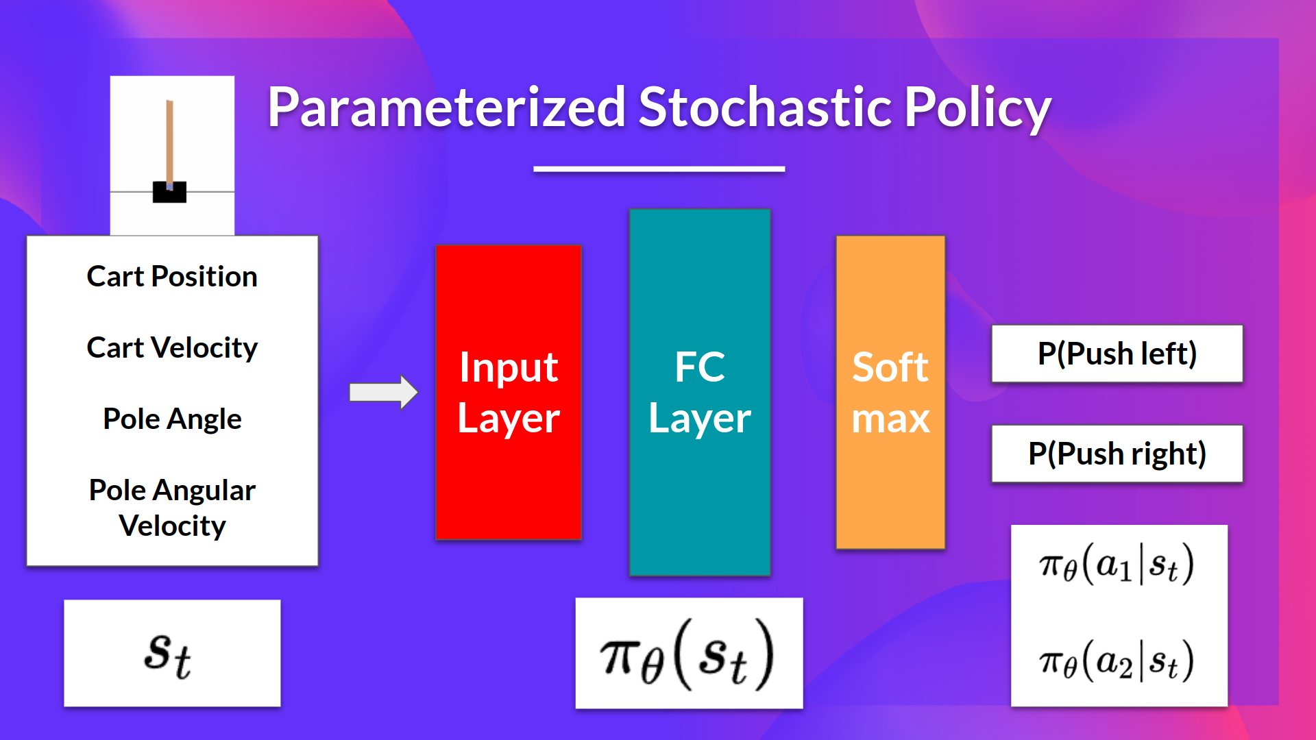
The idea is to parameterize the policy. For instance, using a neural network πθ​, this policy will output a probability distribution over actions (stochastic policy).

Our objective then is to maximize the performance of the parameterized policy using gradient ascent.

To do that, we control the parameter that will affect the distribution of actions over a state.

Consequently, thanks to policy-based methods, we can directly optimize our policy πθ​ to output a probability distribution over actions 𝜋𝜃⟮𝑎

𝑠⟯ that leads to the best cumulative return.

To do that, we define an objective function 𝐽⟮𝜃⟯, that is, the expected cumulative reward, and we want to find the value θ that maximizes this objective function.

---

The difference between policy-based and policy-gradient methods

Policy-gradient methods, what we’re going to study in this unit, is a subclass of policy-based methods. In policy-based methods, the optimization is most of the time on-policy since for each update, we only use data (trajectories) collected by our most recent version of πθ.

The difference between these two methods lies on how we optimize the parameter θ:

• In policy-based methods, we search directly for the optimal policy. We can optimize the parameter θ indirectly by maximizing the local approximation of the objective function with techniques like hill climbing, simulated annealing, or evolution strategies.
• In policy-gradient methods, because it is a subclass of the policy-based methods, we search directly for the optimal policy. But we optimize the parameter θ directly by performing the gradient ascent on the performance of the objective function J(θ).

Before diving more into how policy-gradient methods work (the objective function, policy gradient theorem, gradient ascent, etc.), let’s study the advantages and disadvantages of policy-based methods.

The Advantages and Disadvantages of Policy-Gradient Methods

---

Advantages

The simplicity of integration

We can estimate the policy directly without storing additional data (action values). Policy-gradient methods can learn a stochastic policy

Policy-gradient methods can learn a stochastic policy

Policy-gradient methods can learn a stochastic policy while value functions can’t. This has two consequences:

1. We don’t need to implement an exploration/exploitation trade-off by hand. Since we output a probability distribution over actions, the agent explores the state space without always taking the same trajectory.
2. We also get rid of the problem of perceptual aliasing. Perceptual aliasing is when two states seem (or are) the same but need different actions.

Let’s take an example: we have an intelligent vacuum cleaner whose goal is to suck the dust and avoid killing the hamsters.

Our vacuum cleaner can only perceive where the walls are.

The problem is that the two red (colored) states are aliased states because the agent perceives an upper and lower wall for each.

Under a deterministic policy, the policy will either always move right when in a red state or always move left. Either case will cause our agent to get stuck and never suck the dust.

Under a value-based Reinforcement learning algorithm, we learn a quasi-deterministic policy (“greedy epsilon strategy”). Consequently, our agent can spend a lot of time before finding the dust.

On the other hand, an optimal stochastic policy will randomly move left or right in red (colored) states. Consequently, it will not be stuck and will reach the goal state with a high probability.

Policy-gradient methods are more effective in high-dimensional action spaces and continuous actions spaces

The problem with Deep Q-learning is that their predictions assign a score (maximum expected future reward) for each possible action, at each time step, given the current state. But what if we have an infinite possibility of actions?

For instance, with a self-driving car, at each state, you can have a (near) infinite choice of actions (turning the wheel at 15°, 17.2°, 19,4°, honking, etc.). We’ll need to output a Q-value for each possible action! And taking the max action of a continuous output is an optimization problem itself!

Instead, with policy-gradient methods, we output a probability distribution over actions.

Policy-gradient methods have better convergence properties

In value-based methods, we use an aggressive operator to change the value function: we take the maximum over Q-estimates. Consequently, the action probabilities may change dramatically for an arbitrarily small change in the estimated action values if that change results in a different action having the maximal value.

For instance, if during the training, the best action was left (with a Q-value of 0.22) and the training step after it’s right (since the right Q-value becomes 0.23), we dramatically changed the policy since now the policy will take most of the time right instead of left.

On the other hand, in policy-gradient methods, stochastic policy action preferences (probability of taking action) change smoothly over time.

Disadvantages

Naturally, policy-gradient methods also have some disadvantages:

• Frequently, policy-gradient methods converges to a local maximum instead of a global optimum.
• Policy-gradient goes slower, step by step: it can take longer to train (inefficient).
• Policy-gradient can have high variance. We’ll see in the actor-critic unit why, and how we can solve this problem.

Policy-Gradient Methods

---

The Big Picture

The idea is that we have a parameterized stochastic policy. In our case, a neural network outputs a probability distribution over actions. The probability of taking each action is also called the action preference.

Our goal with policy-gradient is to control the probability distribution of actions by tuning the policy such that good actions (that maximize the return) are sampled more frequently in the future. Each time the agent interacts with the environment, we tweak the parameters such that good actions will be sampled more likely in the future.

But how are we going to optimize the weights using the expected return?

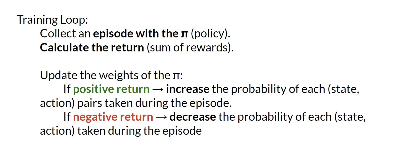
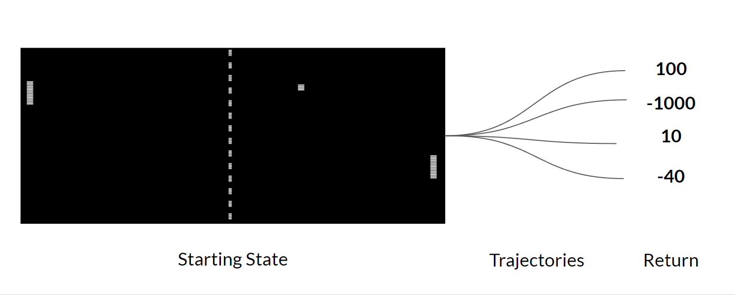
The idea is that we’re going to let the agent interact during an episode. And if we win the episode, we consider that each action taken was good and must be more sampled in the future since they lead to win.

So for each state-action pair, we want to increase the P(a s): the probability of taking that action at that state. Or decrease if we lost.

The Policy-gradient algorithm (simplified) looks like this:

---

We have our stochastic policy π which has a parameter θ. This π, given a state, outputs a probability distribution of actions.

Where πθ(atst) is the probability of the agent selecting action atat​ from state st​ given our policy.

But how do we know if our policy is good? We need to have a way to measure it. To know that, we define a score/objective function called J(θ).

The objective function

The objective function gives us the performance of the agent given a trajectory (state action sequence without considering reward (contrary to an episode)), and it outputs the expected cumulative reward.

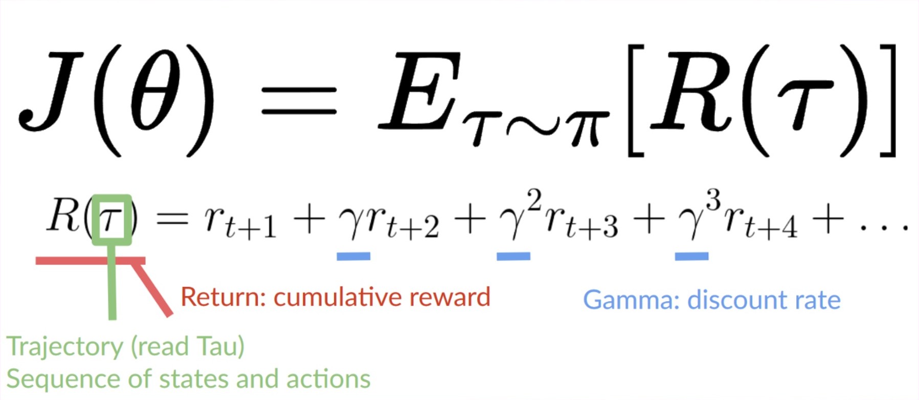
Let’s give some more details on this formula:

The expected return

The expected return (also called expected cumulative reward), is the weighted average (where the weights are given by P(τ;θ) of all possible values that the return R(τ)can take).

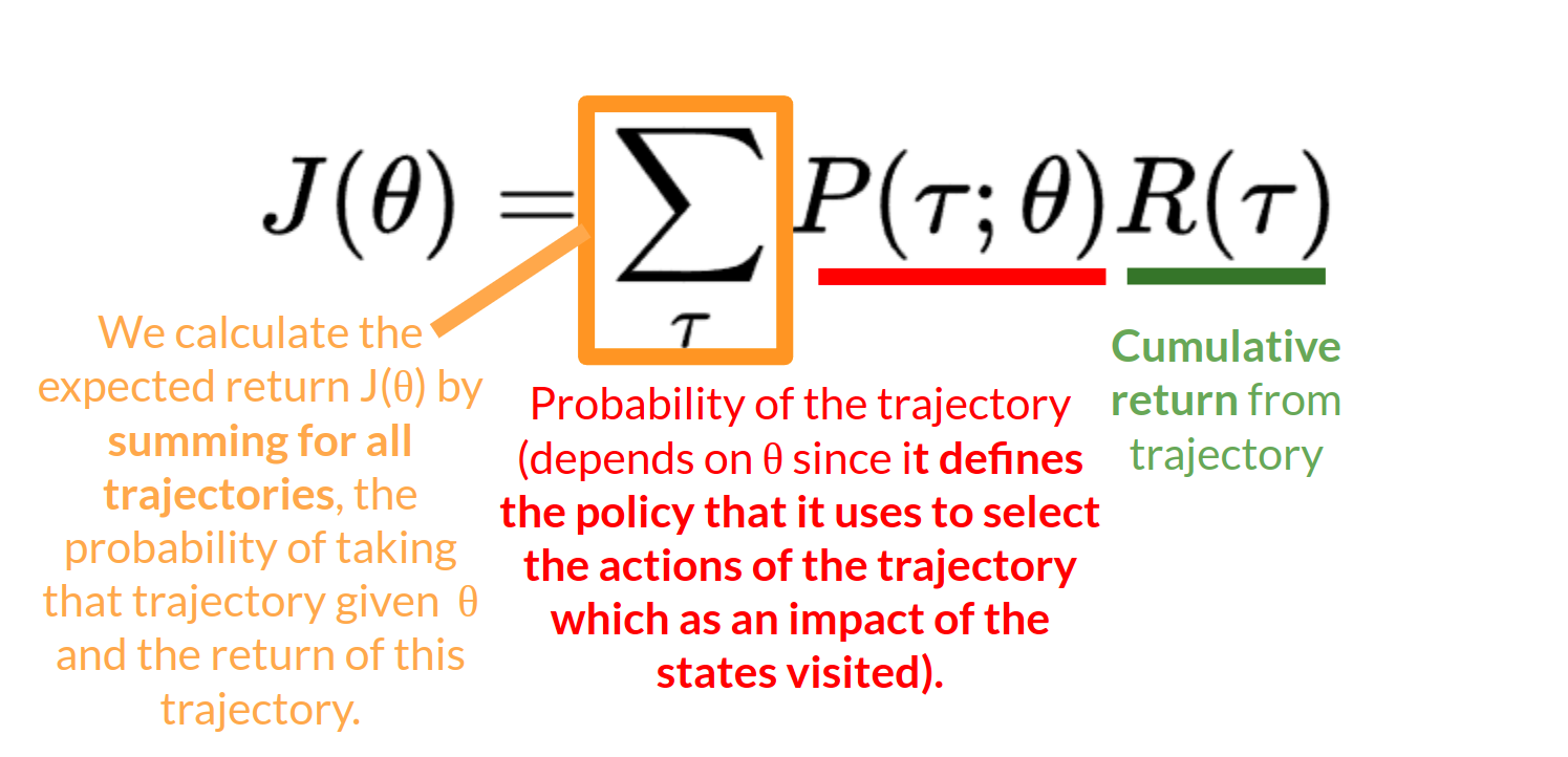
R(τ)

Return from an arbitrary trajectory. To take this quantity and use it to calculate the expected return, we need to multiply it by the probability of each possible trajectory.

P(τ;θ)

Probability of each possible trajectory ττ (that probability depends on θθ since it defines the policy that it uses to select the actions of the trajectory which has an impact of the states visited).

J(θ)

Expected return, we calculate it by summing for all trajectories, the probability of taking that trajectory given θ multiplied by the return of this trajectory.

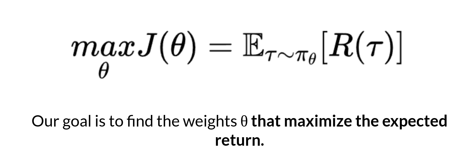
Our objective then is to maximize the expected cumulative reward by finding the θ that will output the best action probability distributions:

The Policy-Gradient Theorem

Policy-gradient is an optimization problem: we want to find the values of θ that maximize our objective function J(θ), so we need to use gradient-ascent. It’s the inverse of gradient-descent since it gives the direction of the steepest increase of J(θ).

Our update step for gradient-ascent is: \(\theta \leftarrow \theta + \alpha * \nabla_\theta J(\theta)\)

We can repeatedly apply this update in the hopes that θ converges to the value that maximizes J(θ).

However, there are two problems with computing the derivative of J(θ):

1. We can’t calculate the true gradient of the objective function since it requires calculating the probability of each possible trajectory, which is computationally super expensive. So we want to calculate a gradient estimation with a sample-based estimate (collect some trajectories).
2. To differentiate this objective function, we need to differentiate the state distribution, called the Markov Decision Process dynamics. This is attached to the environment. It gives us the probability of the environment going into the next state, given the current state and the action taken by the agent. The problem is that we can’t differentiate it because we might not know about it

Fortunately we’re going to use a solution called the Policy Gradient Theorem that will help us to reformulate the objective function into a differentiable function that does not involve the differentiation of the state distribution.

So we have: \(\nabla_\theta J(\theta)=\nabla_\theta \sum_\tau P(\tau;\theta)R(\tau)\)

We can rewrite the gradient of the sum as the sum of the gradient: \(= \sum_\tau \nabla_\theta P(\tau;\theta)R(\tau)\)

We then multiply every term in the sum by \(\frac{ P(\tau;\theta)}{ P(\tau;\theta)}\) (which is possible since it’s = 1)

\[= \sum_\tau \frac{ P(\tau;\theta)}{ P(\tau;\theta)} \nabla_\theta P(\tau;\theta)R(\tau) \\ = \sum_\tau P(\tau;\theta) \frac{\nabla_\theta P(\tau;\theta)}{ P(\tau;\theta)} R(\tau)\]

We can then use the derivative log trick (also called likelihood ratio trick or REINFORCE trick), a simple rule in calculus that implies that: \(\nabla_x log f(x) = \frac{\nabla_x f(x)}{f(x)}\)

So this is our likelihood policy gradient:

\[\nabla_{\theta} J(\theta) = \sum_{\tau} P(\tau;\theta) \nabla_{\theta} \log P(\tau;\theta) R(\tau)\]

Thanks for this new formula, we can estimate the gradient using trajectory samples (we can approximate the likelihood ratio policy gradient with a sample-based estimate if you prefer)

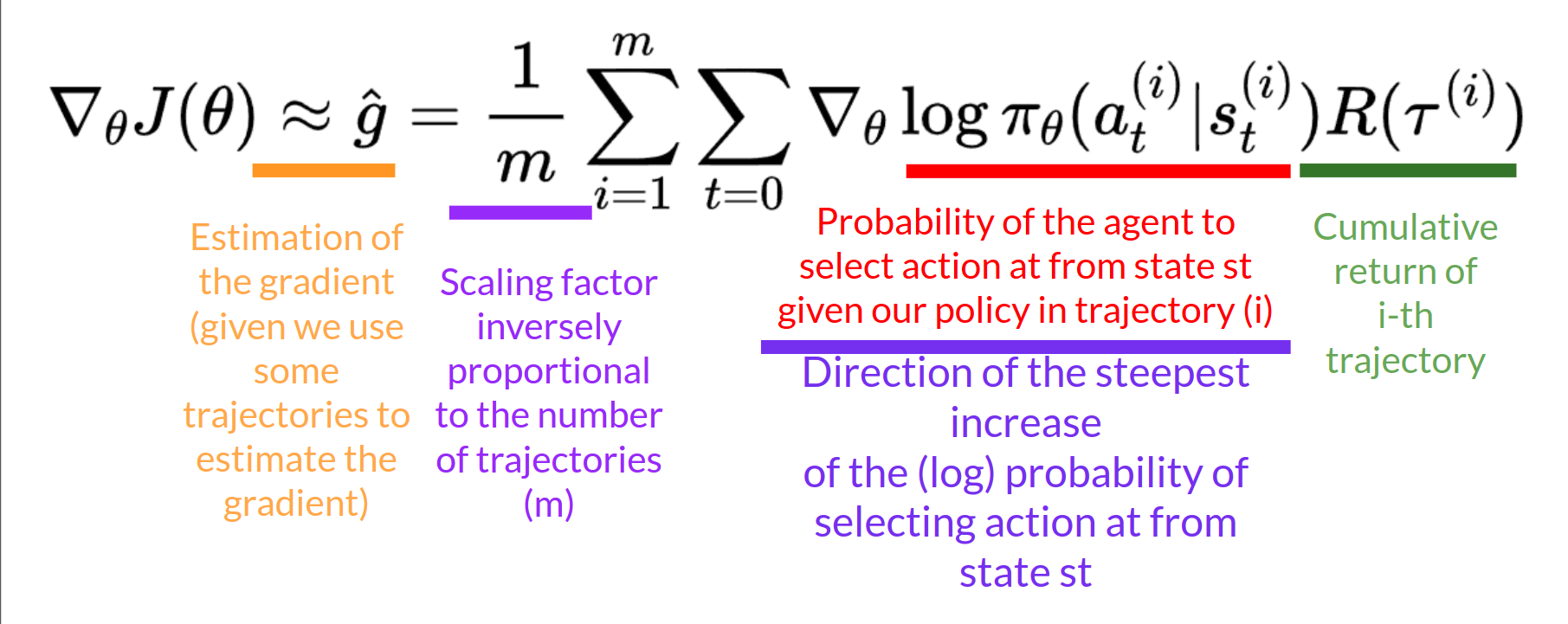
\[\nabla_{\theta} J(\theta) = \frac{1}{m} \sum_{i=1}^{m} \nabla_{\theta} \log P(\tau^{(i)};\theta) R(\tau^{(i)})\]

where each \(\tau(i)\\) is a sampled trajectory.

But we still have some mathematics work to do there: we need to simplify \(\nabla_{\theta} \log P(\tau \mid \theta)\).

We know that:

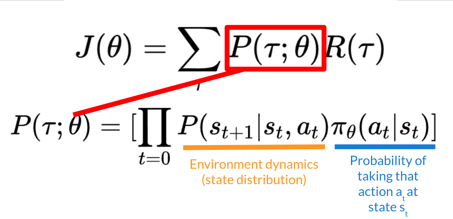
\[\nabla_{\theta} \log P(\tau^{(i)};\theta) = \nabla_{\theta} \log \left[\mu(s_0) \prod_{t=0}^{H} P(s_{t+1}^{(i)} \mid s_t^{(i)}, a_t^{(i)}) \pi_{\theta}(a_t^{(i)} \mid s_t^{(i)})\right]\]

Where \(\mu(s_0)\) is the initial state distribution and \(P(s_{t+1}^{(i)} \mid s_t^{(i)}, a_t^{(i)})\) is the state transition dynamics of the MDP.

We know that the log of a product is equal to the sum of the logs:

\[\nabla_{\theta} \log P(\tau^{(i)};\theta) = \nabla_{\theta} \left[\log \mu(s_0) + \sum_{t=0}^{H} \log P(s_{t+1}^{(i)} \mid s_t^{(i)}, a_t^{(i)}) + \sum_{t=0}^{H} \log \pi_{\theta}(a_t^{(i)} \mid s_t^{(i)})\right]\]

We also know that the gradient of the sum is equal to the sum of gradients:

\[\nabla_{\theta} \log P(\tau^{(i)};\theta) = \\ \nabla_{\theta} \log \mu(s_0) + \nabla_{\theta} \sum_{t=0}^{H} \log P(s_{t+1}^{(i)} \mid s_t^{(i)}, a_t^{(i)}) + \nabla_{\theta} \sum_{t=0}^{H} \log \pi_{\theta}(a_t^{(i)} \mid s_t^{(i)})\]

Since neither the initial state distribution nor the state transition dynamics of the MDP are dependent on (θ), the derivative of both terms is 0. So we can remove them:

Since: \(\nabla_{\theta} \sum_{t=0}^{H} \log P(s_{t+1}^{(i)} \mid s_t^{(i)}, a_t^{(i)}) = 0\) and \(\nabla_{\theta} \mu(s_0) = 0\)

\[\nabla_{\theta} \log P(\tau^{(i)};\theta) = \sum_{t=0}^{H} \nabla_{\theta} \log \pi_{\theta}(a_t^{(i)} \mid s_t^{(i)})\]

We can rewrite the gradient of the sum as the sum of gradients:

\[\nabla_{\theta} \log P(\tau^{(i)};\theta) = \sum_{t=0}^{H} \nabla_{\theta} \log \pi_{\theta}(a_t^{(i)} \mid s_t^{(i)})\]

So, the final formula for estimating the policy gradient is:

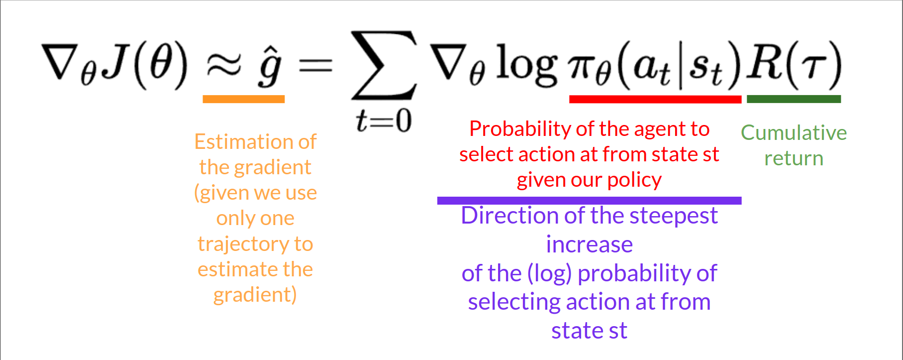
\[\nabla_{\theta} J(\theta) = \hat{g} = \frac{1}{m} \sum_{i=1}^{m} \sum_{t=0}^{H} \nabla_{\theta} \log \pi_{\theta}(a_t^{(i)} \mid s_t^{(i)}) R(\tau^{(i)})\]

The Reinforce Algorithm

The Reinforce algorithm, also called Monte-Carlo policy-gradient, is a policy-gradient algorithm that uses an estimated return from an entire episode to update the policy parameter θ:

In a loop:

• Use the policy \(\pi_{\theta}\) to collect an episode \(\tau\)
• Use the episode to estimate the gradient \(\hat{g} = \nabla_{\theta} J(\theta)\)

• Update the weights of the policy: \(\theta \leftarrow \theta + \alpha \hat{g}\)

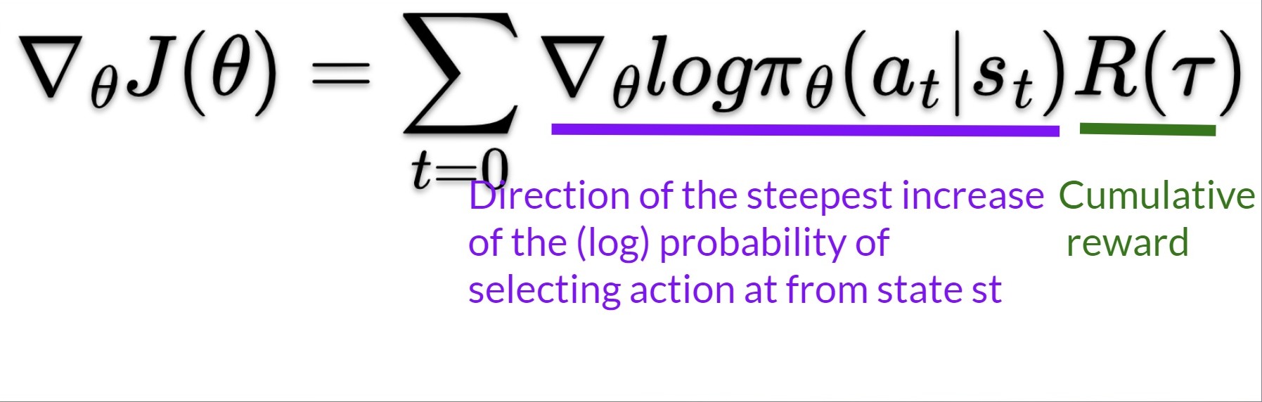
We can interpret this update as follows:

• \(\nabla_{\theta} \log \pi_{\theta}(a_t \mid s_t)\) is the direction of steepest increase of the (log) probability of selecting action \(a_t\) from state \(s_t\). This tells us how we should change the weights of the policy if we want to increase/decrease the log probability of selecting action \(a_t\) at state \(s_t\).
• \(R(\tau)\) is the scoring function:
  • If the return is high, it will push up the probabilities of the (state, action) combinations.
  • Otherwise, if the return is low, it will push down the probabilities of the (state, action) combinations.

We can also collect multiple episodes (trajectories) to estimate the gradient:

The Problem of Variance in Reinforce

In Reinforce, we want to increase the probability of actions in a trajectory proportionally to how high the return is.

• If the return is high, we will push up the probabilities of the (state, action) combinations.
• Otherwise, if the return is low, it will push down the probabilities of the (state, action) combinations.

This return \(R(\tau)\) is calculated using a Monte-Carlo sampling. We collect a trajectory and calculate the discounted return, and use this score to increase or decrease the probability of every action taken in that trajectory. If the return is good, all actions will be “reinforced” by increasing their likelihood of being taken.

\(R(\tau) = R_{t+1}+\gamma R_{t+2}+\gamma^2 R_{t+3} + ...\)

The advantage of this method is that it’s unbiased. Since we’re not estimating the return, we use only the true return we obtain.

Given the stochasticity of the environment (random events during an episode) and stochasticity of the policy, trajectories can lead to different returns, which can lead to high variance. Consequently, the same starting state can lead to very different returns. Because of this, the return starting at the same state can vary significantly across episodes.

We can also collect multiple episodes (trajectories) to estimate the gradient:

Introducing Actor-Critic Methods

In Policy-Based methods, we aim to optimize the policy directly without using a value function. More precisely, Reinforce is part of a subclass of Policy-Based Methods called Policy-Gradient methods. This subclass optimizes the policy directly by estimating the weights of the optimal policy using Gradient Ascent.

We saw that Reinforce worked well. However, because we use Monte-Carlo sampling to estimate return (we use an entire episode to calculate the return), we have significant variance in policy gradient estimation.

Remember that the policy gradient estimation is the direction of the steepest increase in return. In other words, how to update our policy weights so that actions that lead to good returns have a higher probability of being taken. The Monte Carlo variance, which we will further study in this unit, leads to slower training since we need a lot of samples to mitigate it.

So now we’ll study Actor-Critic methods, a hybrid architecture combining value-based and Policy-Based methods that helps to stabilize the training by reducing the variance using:

• An Actor that controls how our agent behaves (Policy-Based method)
• A Critic that measures how good the taken action is (Value-Based method)

---

Reducing variance with Actor-Critic methods

The solution to reducing the variance of the Reinforce algorithm and training our agent faster and better is to use a combination of Policy-Based and Value-Based methods: the Actor-Critic method.

To understand the Actor-Critic, imagine you’re playing a video game. You can play with a friend that will provide you with some feedback. You’re the Actor and your friend is the Critic.

You don’t know how to play at the beginning, so you try some actions randomly. The Critic observes your action and provides feedback.

Learning from this feedback, you’ll update your policy and be better at playing that game.

On the other hand, your friend (Critic) will also update their way to provide feedback so it can be better next time.

This is the idea behind Actor-Critic. We learn two function approximations:

• A policy that controls how our agent acts: \(\pi_\theta (s)\)
• A value function to assist the policy update by measuring how good the action taken is: \(\hat{q}_w(s,a)\)

The Actor-Critic Process

Now that we have seen the Actor Critic’s big picture, let’s dive deeper to understand how the Actor and Critic improve together during the training. As we saw, with Actor-Critic methods, there are two function approximations (two neural networks):

• Actor, a policy function parameterized by theta: \(\pi_\theta (s)\)
• Critic, a value function parameterized by w: \(\hat{q}_w(s,a)\)

Let’s see the training process to understand how the Actor and Critic are optimized:

Step 1:

At each timestep, \(t\), we get the current state \(S_t\) from the environment and pass it as input through our Actor and Critic.

Our Policy takes the state and outputs an action \(A_t\) ​.

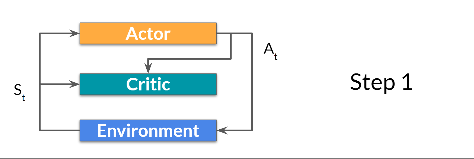
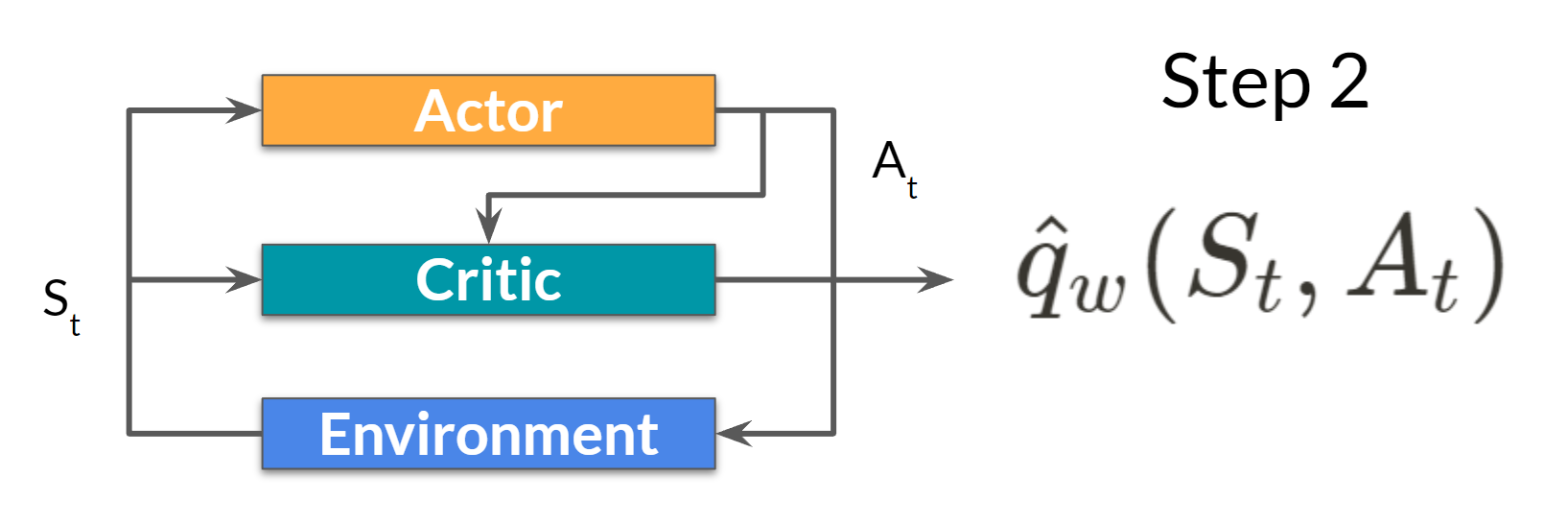
Step 2:

The Critic takes that action also as input and, using \(S_t\) and \(A_t\) computes the value of taking that action at that state: the Q-value.

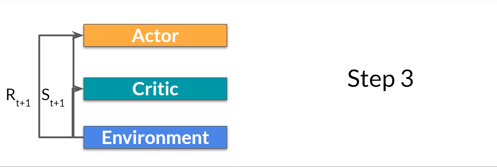
Step 3:

The action \(A_t\) performed in the environment outputs a new state \(S_{t+1}\)​ and a reward \(R_{t+1}\)

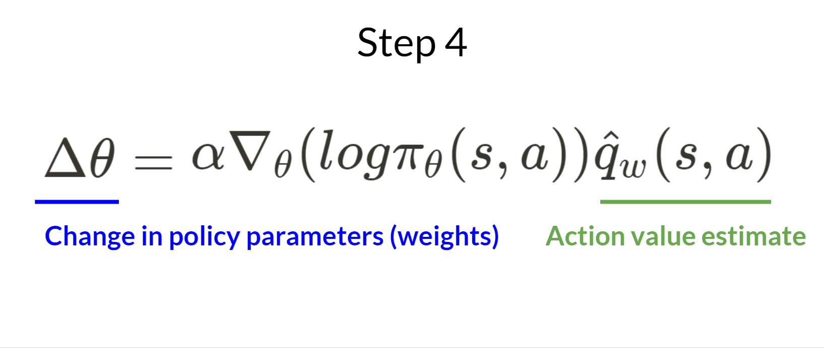
Step 4:

The Actor updates its policy parameters using the Q-value.

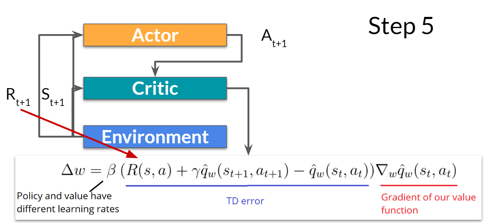
Step 5:

Thanks to its updated parameters, the Actor produces the next action to take at \(A_{t+1}\)​ given the new state \(S_{t+1}\)​.

The Critic then updates its value parameters.

Adding Advantage in Actor-Critic (A2C)

We can stabilize learning further by using the Advantage function as Critic instead of the Action value function.

The idea is that the Advantage function calculates the relative advantage of an action compared to the others possible at a state: how taking that action at a state is better compared to the average value of the state. It’s subtracting the mean value of the state from the state action pair:

In other words, this function calculates the extra reward we get if we take this action at that state compared to the mean reward we get at that state.

The extra reward is what’s beyond the expected value of that state.

• If A(s,a) > 0: our gradient is pushed in that direction.
• If A(s,a) < 0 (our action does worse than the average value of that state), our gradient is pushed in the opposite direction.

The problem with implementing this advantage function is that it requires two value functions — \(Q(s,a)\) and \(V(s)\). Fortunately, we can use the TD error as a good estimator of the advantage function.

Offline vs Online Reinforcement Learning

Deep Reinforcement Learning (RL) is a framework to build decision-making agents. These agents aim to learn optimal behavior (policy) by interacting with the environment through trial and error and receiving rewards as unique feedback.

The agent’s goal is to maximize its cumulative reward, called return. Because RL is based on the reward hypothesis: all goals can be described as the maximization of the expected cumulative reward.

Deep Reinforcement Learning agents learn with batches of experience. The question is, how do they collect it?:

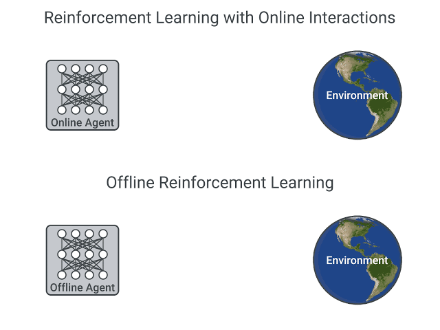
In online reinforcement learning, which is what we’ve learned during this course, the agent gathers data directly: it collects a batch of experience by interacting with the environment. Then, it uses this experience immediately (or via some replay buffer) to learn from it (update its policy).

But this implies that either you train your agent directly in the real world or have a simulator. If you don’t have one, you need to build it, which can be very complex (how to reflect the complex reality of the real world in an environment?), expensive, and insecure (if the simulator has flaws that may provide a competitive advantage, the agent will exploit them).

On the other hand, in offline reinforcement learning, the agent only uses data collected from other agents or human demonstrations. It does not interact with the environment.

The process is as follows:

• Create a dataset using one or more policies and/or human interactions.
• Run offline RL on this dataset to learn a policy

Can we develop data-driven RL methods?

On-policy RL updates the policy while interacting with the environment, off-policy RL learns from data collected by a different behavior policy, and offline RL learns from a fixed dataset without interacting with the environment. Each approach has its own advantages and use cases depending on the specific requirements of the RL problem at hand.

What makes Offline Reinforcement Learning Difficult?

Offline reinforcement learning (RL) presents several challenges that make it a difficult problem to tackle. Here are some of the key factors that contribute to the complexity of offline RL:

Distribution mismatch:

Offline RL involves learning from a fixed dataset of pre-collected experiences, which may not fully represent the dynamics and states of the online environment. There can be a significant difference between the distribution of the offline data and the distribution encountered during training or deployment. This distribution mismatch can lead to poor performance or even instability during the learning process.

Overestimation and extrapolation:

RL algorithms, particularly value-based methods like Q-learning, can be prone to overestimating the values of actions when learning from off-policy data. This issue arises when the behavior policy used for data collection explores different regions of the state-action space compared to the target policy. Overestimation can lead to suboptimal policies and hinder the learning process. Extrapolation errors may also occur when the agent needs to make predictions or take actions in states that were not sufficiently covered in the offline data.

Exploration-exploitation trade-off:

Offline RL lacks the ability to gather new data from the environment to explore and discover better policies. The absence of online exploration makes it challenging to strike the right balance between exploration (gaining knowledge) and exploitation (leveraging existing knowledge). The agent must rely solely on the provided offline dataset, potentially limiting its ability to explore and discover optimal actions in unexplored or uncertain regions of the state-action space.

Data quality and biases:

The quality and biases present in the offline dataset can significantly impact the learning process. The dataset may contain noisy, biased, or suboptimal trajectories, which can mislead the RL algorithm and lead to subpar policies. Identifying and mitigating data quality issues, such as removing outliers or correcting biases, is crucial for effective offline RL.

Stability and safety:

Offline RL algorithms need to ensure stability and safety during the learning process. Without the ability to collect new data and explore, there is a risk of overfitting to the limited offline dataset or encountering catastrophic failures in unfamiliar states. Ensuring stable and safe learning from offline data is a critical concern in offline RL.